[ How to use GPower ] (英語)
※上のサイトは宗教的な内容を含むサイトにありますが、G*Powerの設定の1〜54の全て(Exact, F tests, t tests, χ2tests, Z tests)について網羅していること、それぞれについての設定例をYouTube動画で説明しているため、敢えてリンクをしています。また動画は英語文の解説のみでトークはなくコンパクトで使いやすいこともその理由です。
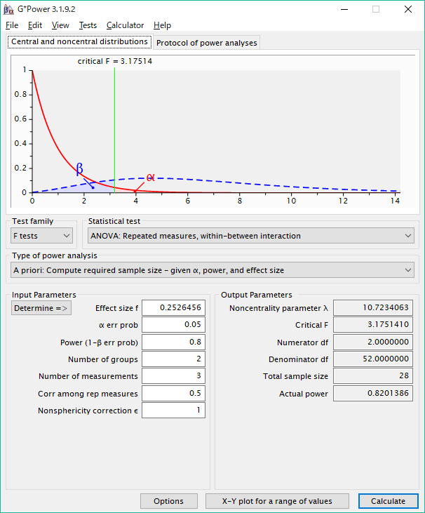
ANOVA: Repeated measures, within-between interaction
(Repeated measures ANOVA [RMANOVA] for testing the interaction between a within subjects variable and a between subjects variable)
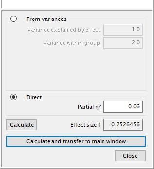
[Detemine]をクリックする(右側に明細を指定する画面が出る)。 "Effect size f" を決めるために、直接法(direct)を選ぶ。「偏イータの 2 乗値」(partial eta squared, partial η2) が、被験者内変数・被験者間変数の相互作用を測るための効果量である。この例では、性別と時期の相互作用によって説明される部分の変動量(variability)を入れる。偏イータ2乗値の近似値は、(効果量)小では0.02、中では0.06,大では0.14である (ここでは 0.06と設定している)。
[Calculte]をクリックすると、効果量"Effect size f"が表示されるので、[Calculate and transfer to main windows]をクリックして、効果量の数値を元の主画面に移行させる。
主画面では、"α err prob"(第一種の過誤または有意水準)の数値を設定する。通常は0.05または0.01である。
"Power (1-β err prob)"には、検定力の数値を入れる。通常は(Cohenの慣例値によると) 0.80である。
"Number of groups" は、被験者間要因(性別)の水準数であり、この例では性別の二値、2である。
"Number of measurements"は、反復測定の回数であり、この例では3つの時期なので3である。
"Corr among rep measures"、すなわち反復測定間の相関では、反復測定の列の間での相関の近似値を入力する。この値は、ある程度の高さのはずである。なぜなら、患者の血液検査の結果は、他の患者達の検査結果と比較すれば時期に関わらずかなり一貫しているはずだからである。この例では、デフォルト値の0.50を用いることにする。
(Repeated measures ANOVA [RMANOVA] for testing the interaction between a within subjects variable and a between subjects variable)
Example: Plan to enroll 16 people (8 women and 8 men) in a study testing effectiveness of a weight loss supplement. Participants’ weights will be measured at 1 month, 2 months, and 3 months. Time is the within subjects variable and gender is the between subjects variable. How many participants are needed to detect a significant interaction between the time variable and gender variable?
Determine Effect Size = Select Procedure -> direct method. Partial eta squared (n2) is the effect size measure for the interaction between the within and between subjects variables. For this example, enter the amount of variability in the outcome that is accounted for by the interaction between gender and time. Approximate partial eta squared conventions are small = .02; medium = .06; large = 0.14.
Click “calculate effect size” and transfer to main window.
α err prob = choose a Type I error rate (usually 0.05 or 0.01)
Power = select a level of statistical power (usually 80% or higher)
Number of groups = levels of the between subjects factor. In this example there are 2 genders.
Number of measurements = number of repeated measures. In this example there are 3 time periods.
Correlation among repeated measures = enter approximate correlation among columns of repeated measures. Note that this value should be somewhat high because patients’ blood test results should be fairly consistent across time relative to other patients’ test results. In this example we’ll use the default value of 0.50.
Nonsphericity correction e = 1.0 if sphericity assumption is met, something else if not met. (Highest value is 1.0, and lowest value = 1/[repetitions - 1].) In the current example we’ll assume this assumption is met (use default value of 1).
What is the Sphericity Assumption? When running repeated measures the variances of the differences between all possible pairs of the within subjects variable should be equivalent. For example, if an outcome variable is measured at time1, time2, and time3, the variances of the differences between time1 - time2, time1 - time3, and time2 - time3 should be roughly the same.
What is the "Nonsphericity correction E" value GPower asks for? This refers to how well the sphericity assumption is met in your data.
Of course this can only be determined with any degree of accuracy if you have preliminary data. If preliminary data are not available and you want to assume that the sphericity assumption will be met, enter 1.0, the default value. If you suspect that your data will deviate from perfect sphericity, enter a value less than 1.0. The more the "nonsphericity correction" drops below 1.0, the more you expect your data to deviate from perfect sphericity. The lowest value GPower allows is 1 / (number of repetitions - 1). One convention holds that a "nonsphericity correction" value should be at least 0.75 or higher in repeated measures ANOVA. If you expect your data to deviate substantially from the sphericity assumption, you may want to use a multivariate method which does not require the sphericity assumption.
What does the “Nonsphericity correction E" value do? When a “nonsphericity correction” value < 1.0 is entered it adjusts the degrees of freedom in the repeated measures ANOVA, resulting in a larger critical value for the test. Larger critical values correct for the lowering of critical values that occurs when the sphericity assumption is not met. In other words, a “nonsphericity correction” value < 1.0 balances out the likelihood of a Type I error that goes up when sphericity is not met. Note that a “nonsphericity correction” value < 1.0 will increase the sample size requirement because it raises the critical cutoff value.